PE-Load Post User Guide
This guide decribes how to evaluate a load simulation project with PE-Load Post. The first steps are explained here:
The next chapters describe how to prepare a evaluation and how to get a look at already existing evaluation results:
At last all evaluation steps and their technical background are explained while the chapter Evaluation Step describes the general procedure for starting evaluation tasks:
User Settings
In the dialog User Settings you have to enter the following credentials to verify your user license.
User
Password
To edit the User Settings at a later point go to File -> User Settings.
Note
After submitting your credentials in User Settings PE-Load Post will verify your license via the PE-Load Post license server. This process requires a working internet connection.
Evaluation
To start an evaluation go to File -> New Evaluation in the menu bar of the main window. In the following dialog you can edit the general properties of the evaluation. These properties (except Simulation Software, Input Top Directory and Output Top Directory) can be altered at any point of an evaluation under Evaluation -> Properties in the menu bar. After accepting this dialog the Input Top Directory (see properties) will be searched for output data from the selected Simulation Software. Every valid load case subdirectory represents a simulation job. In case Adams was selected for Simulation Software a valid load case subdirectory must contain the following files:
Simulation model file (.cmd) which contains meta data about the requests used in the model. Every load case subdirectory found in Input Top Directory must have the same simulation model file.
Result file (.req). Contains output histories data for the requests found in the simulation model file.
(Optional) Flexible bodies files (.for). Contain output histories data for the sections of multiple bodies used in the simulation model. Sections are treated sensor groups.
In case Flex5 was selected the subdirectory must contain the following files:
Result file (.flx5). Contains output histories data for all requested sensors of Flex5 model.
Sensor file (Sensor). Contains meta data of all sensors used in FLex5 model.
In case Fast was selected the subdirectory must contain the following files:
Result file (.out). Contains output histories data for all requested sensors of Fast model.
All valid jobs, sensors and sensor groups found in Input Top Directory will be loaded into the new evaluation.
The evaluation window is seperated in two parts:
Workflow: A tree diagramm displaying all steps of the evaluation process. A double-click on an item (or clicking the respective action Go to <…> in the context menu) opens the respective window in Evaluation Main Window.
Evaluation Main Window: Starting point for the currently selected evaluation step in Workflow. All windows displayed are equally structured (see here) except the Configuration window.
Following evaluation steps are available and can be accessed in window Workflow or in menu View:
Configuration: Edit which jobs and sensors you want to evaluate.
Extract Histories: Extract histories from output folder of the simulation software.
Prepare Histories: Despikes histories, compute moving averages or create new sensor values based on histories of existing sensors.
Extreme Values: Compute contingency table with extreme values from histories.
Extreme Loads: Compute contingency table with extreme values from histories considering partial safety factors.
Extreme Loads (extrapolation): Extrapolates 50year extreme loads.
Extreme Loads (extrapolation, azimuth): Extrapolates 50year extreme loads specifically for Blade Tip Deflections.
Rainflow-Counting: Rainflow-count histories and create job specific Markov matrices.
Load Collective: Aggregate Markov matrices of all included jobs and compute load collective.
DEL: Compute damage equivalent loads based on load collectives.
Regular LDD: Computes load duration distribution. Ranges are based on contingency table with extreme values.
Wind-speed-binned LDD: Computes wind-speed-binned load duration distribution. Ranges are the wind speed bins of the included jobs.
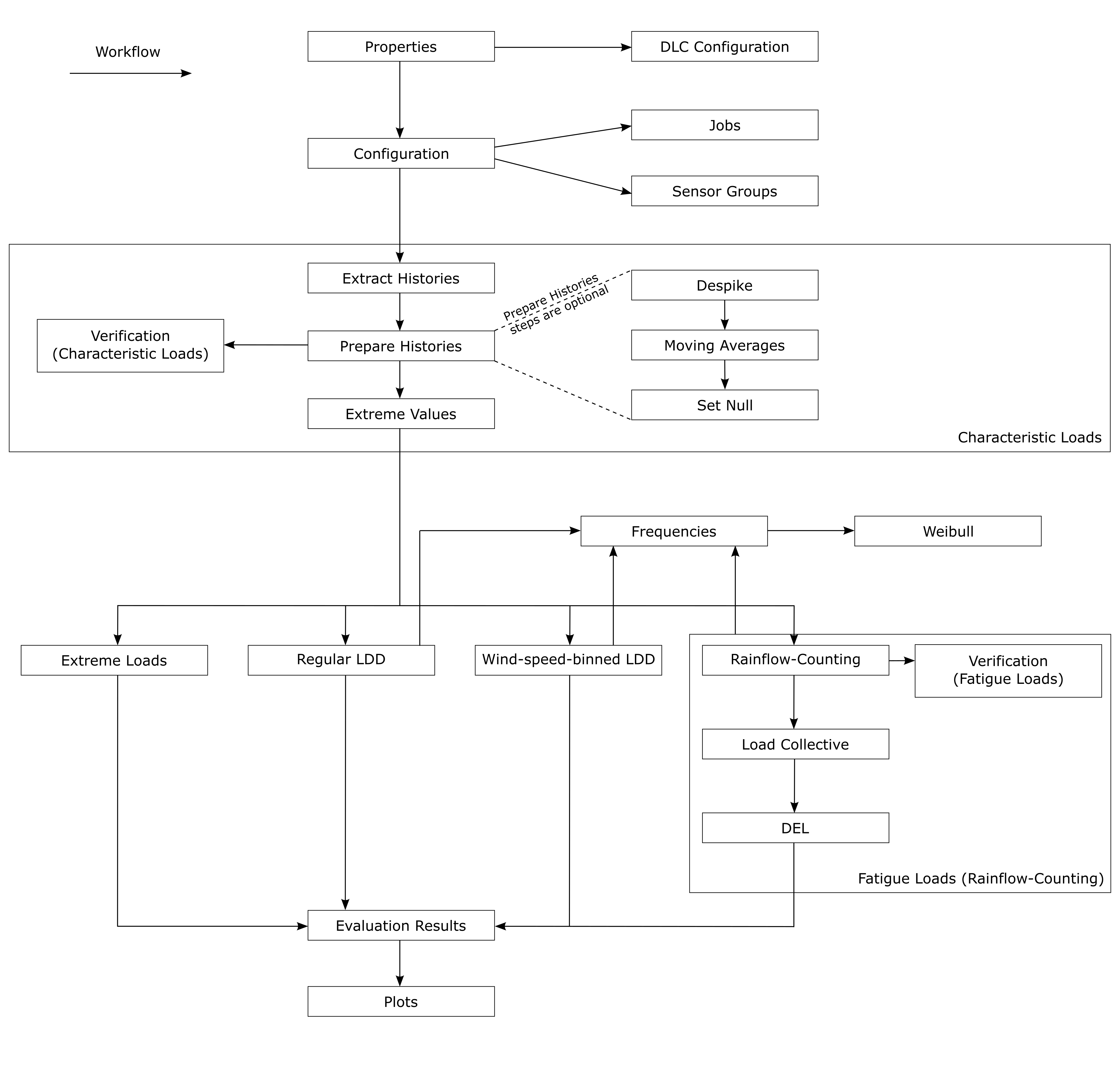
Depending on which kind of analysis you want to do, following sequences of evaluation steps are possible:
Configuration -> Extract Histories -> Prepare Histories -> Extreme Values -> Extreme Loads
Configuration -> Extract Histories -> Prepare Histories -> Extreme Values -> Rainflow-Counting -> Load Collective -> DEL
Configuration -> Extract Histories -> Prepare Histories -> Extreme Values -> Regular LDD
Configuration -> Extract Histories -> Prepare Histories -> Extreme Values -> Wind-speed-binned LDD
Every evaluation step will be executed for all jobs and sensor groups included in window Configuration by the user. The steps Extract Histories, Prepare Histories and Rainflow-Counting will produce an output file for every included job and every included sensor group. The steps Extreme Values, Extreme Loads, Load Collective, DEL, Regular LDD and Wind-speed-binned LDD will produce an output file for every included sensor group.
The following graphic illustrates the workflow of PE-Load Post:
When you save an evaluation under File -> Save Evaluation / File -> Save Evaluation As the following data will be stored as an .eva-file in current directory / given directory (see properties):
Evaluation properties including DLC Configuration.
Weibull properties including current Weibull parameter values and limits.
The job and sensor group data found in Input Top Directory will be saved in a local database (e.g. shelve). Also meta data of all currently existing evaluation results produced by this evalution will be stored in a local database.
An evaluation can be loaded under File -> Load Evaluation. After loading an evaluation you can decide if you want to rescan already existing simulation results to be found in the Input Top Directory and / or rescan evaluation results. Otherwise the evaluation and / or simulation results will be loaded from the local database / shelve.
Evaluation Properties
Parameters
The following evaluation properties can be altered at any point of an evaluation under Evaluation -> Properties.
General Properties:
Evaluation Name: Used et al. as file name for saving Evaluation meta data as .eva file.
Simulation Software: The Simulation Software defines how PE-Load Post interprets the time histories. Can be set to Adams, Bladed, Fast or Flex5.
Input Top Directory: Enter path of top directory under which the histories / output data of the simulation software can be found. Input Top Directory and all its subdirectories will be searched for possible input data.
Output Top Directory: Enter top directory path of evaluation. Evaluation and its results will be stored here.
Evaluation (Misc.) Properties:
Vin: Enter minimum wind speed at which turbine starts production (affects how extrapolation factors are computed for a given weibull distribution, needs to be a positive number).
Vout: Enter maximum wind speed at which turbine stops production (affects how extrapolation factors are computed for a given weibull distribution, needs to be a positive number).
Wind Speed Step Size: Wind speed bin size which affects how extrapolation factors are computed for a given weibull distribution. Needs to be a positive number.
Verification (Characteristic Loads): If checked, Job and Sensor group specific statistics are computed immediatly after the task Prepare Histories.
Verification (Fatigue Loads): If checked, Job and Sensor group specific Load Collectives and DELs are computed immediatly after the task Rainflow-Counting.
Despike Tolerance: Iteration createria for despiking process. A lower value means less iterations are necessary until condition is fulfilled. This will cause a more thorough despiking and a slower despiking process. Needs to be a positive number.
Despike Sigma: Affects threshold over which values are defined as spikes. A lower value means more values will be considered as spikes which will lead to a slower despiking process. Needs to be a positive number.
Despike Max Iteration: Maximum amount of iterations used by Despike algorithm to achieve Despike Tolerance.
Moving Averages Width: Width used for computing moving averages for Prepared Histories.
PSF Fatigue: Partial Safety factor used for all Jobs in a Fatigue Load Analysis. Needs to be a positive number.
Reference Load Cycle Number: Used for Damage Equivalent Load analysis. It is the number of equivalent cycles until failure occurs. Needs to be a positive number.
DEL slope number for Verification (Fatigue Loads): Slope number used for computing Job specific DELs (Verification (Fatigue Loads)).
Number of regular LDD ranges: Number of ranges used for regular Load Duration Distribution analysis. Needs to be a positive integer.
Absolute values for Wind-speed-binned LDD: Check / uncheck if only absolute values are considered for Wind-speed-binned LDD analysis.
Decimal precision: Number of decimal points used for data produced by PE-Load Post. Needs to be a positive integer.
Number of usable CPUs: Number of available CPUs used for computing Evaluation Tasks.
Number of usable CPUs for Extracting Histories: Number of available CPUs used for Extracting Histories. This task is limited by read / write performance of the storage drive. Using too many CPUs might slow down performance.
Regex for capturing DLC name: Regular Expression string for capturing DLC name from Job name (see DLC Configuration).
Evaluation (Extreme Extrapolation) Properties
Moving Window: Width of moving window in seconds to extract local extrema.
Azimuth Min: Minimum of azimuth angle in degrees for filtering data.
Azimuth Max: Maximum of azimuth angle in degrees for filtering data.
Bootstrap Resamplings: Number of bootstrap resamplings to determine confidence intervals. A minimum number of 25 bootstrap resamplings may be sufficient to determine a reasonable estimate of confidence bounds. However, a larger number closer to 5 000 will lead to more reliable estimates.
Max Shape Parameter: Maximum of shape parameter of fitted distribution: Should equal -0.1 for generalized pareto distribution.
Exceedance Probability: Exceedance probability for characteristic extremum (Should equal 3.8e-07 for 50 years according IEC 61400-1).
Force Extrapolation: Force extrapolation by skipping bins with unsatisfying fitting criteria , if extrapolation does not converge.
To test your Regular Expression go to RegExp Tester.
DLC Configuration
In the dialog DLC Configuration you can specify group specific evaluation properties which will be applied to all jobs of the respective DLC:
Group: Name of DLC. Jobs whose name contain the value Group (property Regex for capturing DLC name is used to extract DLC name from job name) will be assigned to this Group.
Settling: Settling-in time is the time period at the beginning of every job which will not be included in evaluation.
Duration: Duration plus Settling should equal total job time.
Factor_Extreme: Partial Safety Factor used for Extreme Loads analysis.
- Type: Comma separated list of identifiers to specify which analysis types should be used for the respective DLC:
F: Fatigue Load analysis.
U: Extreme Load analysis. Max/min values are highest/lowest values of all jobs.
U_mw: Extreme Load analysis. Max/min values are computed as means of max/min values of all jobs.
U_umw: Extreme Load analysis. Max/min values are computed as means of 50% of the jobs that have the highest/lowest max/min values.
Additionally you can import / export DLC configurations (.dlc file).
Weibull Distribution
Under Evaluation -> Weibull Distribution in the main window menu bar the values and properties of the Weibull distribution can be edited. This distribution can be used for setting the extrapolation factors necessary for weighing the jobs in the Load Collective, Regular LDD and Wind-speed-binned LDD analysis.
For every wind speed bin (from 0 to 50 m/s) the relative frequency \(h_{v}\) can be manually set. Further the Weibull distribution and its relative frequencies can be created by applying the Weibull formula
\(h_{v}(v) = e^{-(\frac{v - 0.5 \Delta v }{\lambda})^k} - e^{-(\frac{v + 0.5 \Delta v}{\lambda})^k}\)
which is based on the cumulative distribution function and where \(k\) is the Weibull shape parameter, \(\lambda\) the Weibull scale parameter, \(v\) the respective wind speed bin and \(\Delta v = 1 \frac{m}{s}\) the wind speed bin step size. To apply the formula click on Apply Formula. Here the Weibull shape and scale parameters can be edited. The check box Formula Used indicates whether the current Weibull distribution values \(h_{v}\) correspond with the current Weibull formula defined by the Weibull parameters displayed above the check box. Under Frequency Sum (-) the sum of all \(h_{v}\) values of the distribution is displayed (the sum should be approximately 1).
Under Limits you can determine whether the probabilities for wind speed bins under \(v_{in}\) and above \(v_{out}\) should be added to the wind speed bins \(v_{in}\) and \(v_{out}\) or be disregarded.
Frequencies
To edit the job frequencies open the windows for Rainflow-Counting, Load Collective, DEL, Regular LDD or Wind-speed-binned LDD analysis by double-clicking on the respective entry in the window Workflow or by clicking to the respective entry in menu View of the main window menu bar. Then go to Set Frequencies for included Jobs in the context menu of the evaluation main window. The following dialog enables the user to set the frequencies of all currently included jobs (that is all jobs included for the respective evaluation step). This dialog is also opened every time before evaluation tasks including Load Collective, Regular LDD or Wind-speed-binned LDD analysis are about to be processed.
By assigning frequencies to the jobs and their respective job groups PE-Load Post can compute extrapolation factors based on the frequencies, job specific simulation durations and Lifetime in Years of the wind turbine. In this dialog the user can edit the Lifetime in years of the wind turbine and the relative frequency \(h_{j}\) of every group of the included jobs in column Group Frequency hj (-). Further the user can determine which way the relative job frequencies should be entered in the column Frequency Type. Following Frequency Types are available:
Weibull: User edits Weibull distribution from which the job frequencies will be derived.
Duration: User enters total duration (in hours) per year for every job.
Absolute Frequency: User enters total number of events per Lifetime in years for every job.
Relative Frequency: User enters relative job frequency within the group for every job.
Under Frequency Sum (-) the sum of all relative group frequencies \(h_{j}\) is displayed. This sum should be approximately 1. In the same way the relative frequencies h_{v} of the Weibull distribution and the directly entered relative job frequencies h_{i) (Relative Frequency) should sum up approximately to 1. To edit the relative job frequencies within a group click on the button in the respective row of the group.
In the following the calculation process of the frequencies and the extrapolation factors is explained. The job frequencies are computed by multiplying the relative frequency \(h_{j}\) of the group \(j\) with the relative frequency \(h_{i}\) of the job \(i\) within the group:
\(h_{i,j} = h_{i} h_{j}\)
The extrapolation factor \(p_{i,j}\) is obtained with
\(p_{i,j} = \frac{h_{i,j}T}{t_{i,j}}\)
where \(T\) is wind turbine lifetime and \(t_{i,j}\) is the simulation duration of the respective job.
The relative group frequency \(h_{j}\) is entered directly while the job frequency \(h_{i}\) can be entered in 4 different ways:
Derived from the Weibull distribution based on the wind speed \(v_{hub}\) of the job.
Enter total duration of job \(T_{i,j}\) per year. In this case the relative group frequency \(h_{j}\) is indirectly computed and cannot be altered.
Enter total number job events \(H_{i}\) per Lifetime in Years. In this case the relative group frequency \(h_{j}\) is indirectly computed and cannot be altered either.
Enter relative job frequency \(h_{i}\) directly.
For the cases 1 and 4 the sum of the relative job frequencies \(h_{i}\) will always be rounded up to 1 although the actual sum of the job frequencies that were derived from the Weibull distribution (1) or entered directly (4) may not be 1.
For the case 1 the relative job frequency \(h_{i}\) will be derived from the Weibull distribution. The bigger the evaluation property Wind Speed Step Size is the bigger will be the derived relative job frequency. Following example explains the calculation of an extrapolation factor for a job based on a Weibull distribution:
The wind speed of a job \(i\) is \(v_{hub,i} = 8\) and the relative frequencies per wind speed in the Weibull distribution are
\(h_{v}(v_{hub}=7) = 0.12\),
\(h_{v}(v_{hub}=8) = 0.10\) and
\(h_{v}(v_{hub}=9) = 0.08\).
If the Wind Speed Step Size is 2 then the relative job frequency will be:
\(h_{i}(v_{hub}=8) = 0.5 \cdot 0.12 + 1 \cdot 0.10 + 0.5 \cdot 0.08 = 0.2\)
If the Wind Speed Step Size is 1.5 then the relative job frequency will be:
\(h_{i}(v_{hub}=8) = 0.25 \cdot 0.12 + 1 \cdot 0.10 + 0.25 \cdot 0.08 = 0.15\)
Now if Wind Speed Step Size is 2 and the relative frequency of the group \(j\) to which job \(i\) belongs is \(h_{j} = 0.3\) then the total frequency of the job is:
\(h_{i,j} = h_{i} h_{j} = 0.3 \cdot 0.2 = 0.06\)
Assuming that the Lifetime in Years is 20 and the simulation duration of the job is 600 seconds then the extrapolation factor will be:
\(p_{i,j} = \frac{h_{i,j}T}{t_{i,j}} = \frac{0.06 \cdot 20 \cdot 365 \cdot 24}{\frac{600}{3600}} = 63072\)
Evaluation Results
To open the Evaluation Results dialog go to View -> Evaluation Results in the menu bar. In this dialog all results created by this evaluation are displayed. Under the context menu you can open / delete the respective evaluation result file and / or the directory of the file.
Note
Always delete evaluation results from the dialog Evaluation Results so the respective entries in the database can be deleted along the files themselves. Avoid deleting evaluation result files manually.
Extracted histories and prepared histories are stored as Numpy binaries (e.g. with .npy extension). Additionally to every numpy binary a file with meta data is created (e.g. with .history / .despiked extension). To convert and / or open binary files created by PE-Load Post open the Evaluation Results dialog or go to File -> Convert Binary Histories or File -> Convert and Open Binary Histories in the menu bar.
To plot evaluation results go to Plot. In the following dialog you can configure which sensors from which jobs PE-Load Post should plot. Additionally you can decide in how many subplots the plot should be divided and which results should be displayed in which subplots. The configuration table consists of the following columns:
Plot / Label: Name of subplot and labels for results displayed within the respective subplots.
Sensor: Sensor name of result to be plotted.
Job: Job name of result.
Sensor Group: Sensor Group name of result.
Source: Source name of result. Source can be the current Evaluation or any evaluation result file compatible with PE-Load Post.
To add a subplot go to Add Plot. To add a result of the current evaluation to a subplot go to Add Sensor, to add a result from any evaluation result file compatible with PE-Load Post go to Add Sensor From File. To change the plot order go to ‘<’ or ‘>’, to remove a subplot or a sensor / result from a subplot go to Remove.
To show statistical analysis results (see Verification (Characteristic Loads) / Verification (Fatigue Loads), they can be activated / deactivated) created during the evaluation steps Prepare Histories and Rainflow-Counting go to Plot Statistic in the dialog Evaluation Results (in tabs Prepared Histories and Rainflow-Counted).
Configuration
The evaluation process starts with the Configuration. You can access it by double-clicking on Configuration in the Workflow window or under the respective entry in menu View of the manu bar. Following two tabs display the simulation output data found in Input Top Directory:
Jobs: List of all jobs (load cases) segmented by their DLC group. Here you can select all jobs you want to include in the evaluation.
- Sensor Groups: List of all sensor groups and sensors. You can create, edit and delete sensor groups and sensors. The following columns define a sensor / sensor group:
Name: Name of sensor / sensor group used for the evaluation and displayed in evaluation result files (must be a unique name).
Value: Name of sensor within the respective simulation software (e.g. Fast). Names are formatted as <sensor_group_name>.<sensor_name>. All possible sensor names are defined in the respective input file in PE-Load Post directory (e.g. /data/fast/fast_requests.txt). If two sensor values separated by the character ‘:’ are specified, the values of the sensor will be computed as geometric means of the two specified sensor values. For more info on geometric mean calculation, see Prepare Histories.
- You can select all sensors / sensor groups you want to include for one or more of the following analysis options:
Characteristic Loads, Includes Extract Histories, Prepare Histories and Extreme Value analysis.
Prepare Histories: Despike, Despikes sensor values when step Prepare Histories is processed.
Prepare Histories: Moving Avg, Computes moving averages of sensor values when step Prepare Histories is processed.
Prepare Histories: Set Null, Sets all sensor values to 0 when step Prepare Histories is processed.
Extreme Loads, Includes a Extreme Loads analysis.
Fatigue Loads(Rainflow), Includes Rainflow-Counting, Load Collective and DEL analysis
Fatigue Loads (regular LDD), Includes Regular LDD fatigue analysis.
Fatigue Loads (wind-speed-binned LDD), Includes Wind-speed-binned LDD fatigue analysis.
For all tabs several filter options (below table) and editing options (under context menu) are available. For example in tab Jobs you can include / exclude jobs by selecting / deselecting their groups under Include / Exclude Job Groups in the context menu.
Evaluation Step
Every evaluation step displayed in the main window of the evaluation except Configuration is similarly structured. All jobs (segmented by their groups) that were included in Configuration are displayed.
For each job you can decide if you want to actually include it for the analysis of this evaluation step. All jobs that have the same analysis type (see DLC Configuration) as the analysis type of the current evaluation step (Fatigue Load analysis, Extreme Load analysis, etc.) are automatically included at first. Evaluation steps for Characteristic Load analysis are always automatically included.
Further the PSF Fatigue value is displayed for fatigue evaluation steps and the job specific extreme load PSF from the job interface file is displayed for extreme load evaluation steps.
At last for each job you can see to which step the evaluation has arrived. If the current status of job DLC1p1_NTM7p0mps_Y00_RS0016010 is Extreme Values Extracted it means that for all sensor groups that are included for a Characteristic Load analysis, the evaluation steps Extract Histories, Prepare Histories and Extreme Values already have been processed for this job.
Several filter options (below table) and editing options (under context menu) are available. Following options are available among others in the context menu:
Start evaluation tasks for all included jobs (
 action).
Include / exclude jobs by selecting / deselecting their groups (Include / Exclude Job Groups).
Rescan all evaluation results (Rescan Evaluation Results).
Show and edit all evaluation results (Show Evaluation Results).
After clicking on the action in the context menu the dialog Select Starting Process will be opened. Here you can decide for every job with which evaluation step the evaluation process should start.
Several filter options (below table) and editing options (under context menu) are available as well. The combo box in column Start With Process in the respective row displays all possible starting processes.
After clicking on Continue the next dialog Evaluation Tasks will be opened. It shows all evaluation tasks that are about to be processed. For each evaluation task the follwing infos are displayed:
Task (for example Extract Histories, Prepare Histories, etc.)
Job
Sensor Group
Already Evaluated (true if evaluation task already has been processed and therefore the according evaluation result file already exist)
If already evaluated results exist you can decide to revaluate the already evaluated tasks or ignore them by clicking the check box Replace already existing Results.
After clicking on Continue all designated evaluation tasks will be sequentially processed. Following example clarifies the procedure:
We open window Extreme Values by double-clicking on Extreme Values in the Workflow window. We only include the hypothetical job DLC1p1_NTM7p0mps_Y00_RS0016010 and start an evaluation task run by clicking on Compute Extreme Values in the context menu. Subsequently the dialog Select Starting Process will be opened. If in the row of DLC1p1_NTM7p0mps_Y00_RS0016010 the combo box in column Start With Process has the entries Extract Histories and Prepare Histories it means that for all included sensor groups included for Characteristic Load analysis in window Configuration the evaluation step Extract Histories already has been processed. However the evaluation step Prepare Histories has not been processed yet at least not for all included sensor groups included for Characteristic Load analysis. If we select the entry Extract Histories and assume that we included the sensor group Bladed_tip_node_1 and crs_tower_1001 for Characteristic Load analysis in Configuration then the following tasks in the displayed order are about to be processed:
Task |
Job |
Sensor Group |
|---|---|---|
Extract Histories |
DLC1p1_NTM7p0mps_Y00_RS0016010 |
Bladed_tip_node_1 |
Extract Histories |
DLC1p1_NTM7p0mps_Y00_RS0016010 |
crs_tower_1001 |
Prepare Histories |
DLC1p1_NTM7p0mps_Y00_RS0016010 |
Bladed_tip_node_1 |
Prepare Histories |
DLC1p1_NTM7p0mps_Y00_RS0016010 |
crs_tower_1001 |
Extract Extreme Values |
DLC1p1_NTM7p0mps_Y00_RS0016010 |
Bladed_tip_node_1 |
Extract Extreme Values |
DLC1p1_NTM7p0mps_Y00_RS0016010 |
crs_tower_1001 |
If we select for job DLC1p1_NTM7p0mps_Y00_RS0016010 the entry Prepare Histories in column Start With Process in dialog Select Starting Process then following tasks in the displayed order are about to be processed:
Task |
Job |
Sensor Group |
|---|---|---|
Prepare Histories |
DLC1p1_NTM7p0mps_Y00_RS0016010 |
Bladed_tip_node_1 |
Prepare Histories |
DLC1p1_NTM7p0mps_Y00_RS0016010 |
crs_tower_1001 |
Extract Extreme Values |
DLC1p1_NTM7p0mps_Y00_RS0016010 |
Bladed_tip_node_1 |
Extract Extreme Values |
DLC1p1_NTM7p0mps_Y00_RS0016010 |
crs_tower_1001 |
Note
If a Extract Histories or Prepare Histories task finishes and an old result file for same the job and sensor group already exists, the old file will be overwritten. For evaluation task type Compute DEL old files will be overwritten if they contain results for the same sensor group and load cycle number. For all other types of evaluation tasks (e.g. Extract Extreme Values, Rainflow-Counting etc.) old files will be overwritten if they contain results for the same sensor group.
Extract Histories
You can access this evaluation step by double-clicking on Extract Histories in the Workflow window or under the respective entry in menu View of the menu bar.
It will extract the histories for the included jobs in this window and for included sensor groups included for Characteristic Load analysis in Configuration from the Input Top Directory. The extracted histories will be stored as Numpy binaries (e.g. with .npy extension).
The extracted histories can be found in the directory /temp/histories of the Output Top Directory. To convert them to Ascii format see evaluation_results. Here is an example
of an extracted history file for a load sensor group converted to Ascii format.
Prepare Histories
You can access this evaluation step by double-clicking on Prepare Histories in the Workflow window or under the respective entry in menu View of the menu bar.
It will despike the histories for the included jobs in this window and for sensors included for Prepare Histories: Despike analysis in Configuration based on the parameters Despike Tolerance, Despike Sigma and Despike Max Iteration in the properties. It will compute the moving averages for sensors included for Prepare Histories: Moving Avg analysis in Configuration. It will set all values to zero for sensors included for Prepare Histories: Set Null analysis in Configuration. Further the histories will be cut based on the parameters Settling and Duration in DLC Configuration. If the Value of a sensor in Configuration is two sensor values separated by the character ‘:’ it will compute the geometric means of histories of the specified two sensors.
The despiked histories will be stored as Numpy binaries (e.g. with .npy extension). If the option Verification (Characteristic Loads) has been selected, for every sensor group a file will be created that contains job specific statistics.
The despiked histories can be found in the directory /temp/despiked_histories of the Output Top Directory. To convert them to Ascii format see evaluation_results.
The sensor group specific statistic file can be found under /temp/despiked_histories as well. Here is an example
of a despiked history file for a sensor group converted to Ascii format.
Here is an example of a statistics file for a load sensor group.
Despike
In the following the despiking process for a column with the values \(x(t)\) is described. First the derivative \(\Delta x(t)\) for every time step is computed. Then the standard deviation \(\sigma_{\Delta x}\) of the time derivated values is determined. Based on the property parameter Despike Sigma it will now be verified if a value \(x_{i}\) is a spike or not. It is a spike if following condition is met:
\(|\Delta x_{i}| > k \cdot \sigma_{\Delta x}\)
Here \(k\) is the parameter Despike Sigma. Further a value \(x_{i}\) will be despiked if one of the four preceding values \(x_{i-4}...x_{i-1}\) or one of the four succeeding values \(x_{i+1}...x_{i+4}\) are spikes. Now for all determined spikes the despiked values \(x_{i,d}\) will be computed based on the moving averages principle:
\(x_{i,d} = x_{i-4} + (x_{i+4}-x_{i-4}) \frac{t_{i}-t_{i-4}}{t_{i+4}-t_{i-4}}\)
Here \(x_{i-4}\) is the value four steps before \(x_{i}\) while \(x_{i+4}\) is the value four steps after \(x_{i}\). Further \(t_{i}\), \(t_{i-4}\) and \(t_{i+ 4}\) are the corresponding time steps of \(x_{i}\), \(x_{i-4}\) and \(x_{i+4}\).
Now once again the time derivative \(\Delta x_{d}(t)\) and its standard deviation \(\sigma_{\Delta x_{d}}\) of the despiked values \(x_{d}(t)\) are computed and checked if the following iteration condition is met:
\(|\frac{\sigma_{\Delta x_{d}}}{{\sigma_{\Delta x}}}| - 1 <= c\)
Here \(c\) is the evaluation property Despike Tolerance, \(\sigma_{\Delta x}\) is the old standard deviation and \(\sigma_{\Delta x_{d}}\) is the new standard deviation. If this iteration condition is met then the despiking process for this column ends. Otherwise the whole process described above will be repeated again until the iteration condition is met or until the maximum amount of despike iterations have been done.
Moving Averages
The moving averages for a sensor are computed based on the following equation
\(x_{i} = \frac{x_{i-n}+x_{i-(n-1)}+...+x_{i}+...+x_{i+(n-1)}+x_{i+n}}{ 2n + 1}\)
where \(x_{i}\) is the filtered value and \(n\) is the Moving Averages Width.
Geometric means
The geoemetric means of two sensor histories are computed based on the following equation
\(F_{12} = \sqrt{F_{1}^2 + F_{2}^2}\)
where \(F_{1}\) and \(F_{2}\) are the input values of the respective sensors and \(F_{12}\) the geometric mean.
Extreme Values
You can access this evaluation step by double-clicking on Extreme Values in the Workflow window or under the respective entry in menu View of the menu bar.
It will compute the contingency table of extreme values (without considering PSF) for the included jobs in this window and for included sensor groups included for Characteristic Load analysis in Configuration. While the preceding evaluation steps (Extract Histories and Prepare Histories) were job specific this step aggregates results of all included jobs. So for every included sensor group a extreme value file will be created.
The extreme values can be found in the directory /temp/extreme_values of the Output Top Directory. Here is an example
of an extreme value file for a load sensor group.
Extreme Loads
You can access this evaluation step by double-clicking on Extreme Loads in the Workflow window or under the respective entry in menu View of the menu bar.
It will compute the contingency table of extreme loads (considering job specfic PSF) for the included jobs in this window and for included sensor groups included for Extreme Load analysis in Configuration. This step aggregates results of all included jobs. For every included sensor group a extreme load file will be created.
The extreme loads can be found in the directory /ult/extreme_loads of the Output Top Directory. Here is an example
of an extreme load file for a load sensor group.
Rainflow-Counting
You can access this evaluation step by double-clicking on Rainflow-Counting in the Workflow window or under the respective entry in menu View of the menu bar.
It will run a rainflow-counting and compute the respective Markov matrices for the included jobs in this window and for the included sensor groups included
for Fatigue Load (Rainflow) analysis in Configuration. This step is executed with NREL Crunch. The column specific ranges are determined by the max-min-ranges
computed in the preceding evaluation step Extreme Values. For further information see the Crunch manual. If the option Verification (Fatigue Loads) has been selected, for every
sensor group the Job specific DELs will be computed for a given DEL slope number.
The Markov matrices can be found in the directory /temp/markov of the Output Top Directory. The Job specific DELs are aggregated for all included sensor groups and can be found under /temp/markov as well. Here is an example
of a Markov file and aggregated DEL file for a load sensor group.
Load Collective
You can access this evaluation step by double-clicking on Load Collective in the Workflow window or under the respective entry in menu View of the menu bar.
It will compute the load collectives (considering PSF Fatigue) for the included jobs in this window and for the included sensor groups included for Fatigue Load (Rainflow) analysis in Configuration. This step aggregates results of all included jobs. For every included sensor group a load collective file will be created. Further for every load collective analysis the aggregated matrices and the job frequencies (including extrapolation factors) used for computing the load collectives are written into a respective file as well.
The aggregated Markov matrices can be found in the directory /fat/markov_aggregated of the Output Top Directory. Here is an example
of a file with aggregated matrices for a load sensor group.
The applied job frequencies can be found in the directory /fat/collective of the Output Top Directory. Here is an example
of a file with the applied job frequencies for a load sensor group.
The load collectives can be found in the directory /fat/collective of the Output Top Directory. Here is an example
of a load collective file for a load sensor group.
In the following the process of computing the load collective of a dimension is described. First the Markov matrices from every included job computed in the preceding evaluation step Rainflow-Counting are aggregated. This is possible since all Markov matrices have the same ranges which were extracted from the preceding step Extreme Values for the same job combination that is used for this evaluation step. Before aggregating the matrices the values of the matrices will be multiplied with the extrapolation factor (based on the job frequency) of the respective job.
After the matrices have been aggregated for a dimension the column \(n_{i}\) will be computed. Each entry is the sum of all events found in one range (row) \(i\) of the aggregated Markov matrice. At last the column \(N_{i}\) will be computed. It contains the cumulated values of column \(n_{i}\) beginning with the value in the highest range of the respective dimension.
DEL
You can access this evaluation step by double-clicking on DEL in the Workflow window or under the respective entry in menu View of the menu bar.
It will compute the damage equivalent loads (considering PSF Fatigue) for the included jobs in this window and for the included sensor groups included for Fatigue Load (Rainflow) analysis in Configuration. As the preceding step Load Collective already aggregated all included jobs the evaluation step DEL will produce an output file for every included sensor group.
Before starting a DEL analysis the user has to enter the Load Cycle Number \(N_{ref}\). If a DEL file based on the same \(N_{ref}\) value already exist then it will be overwritten. Otherwise the current DEL file will just be added to the other already existing DEL files based on other \(N_{ref}\) values.
The damage equivalent loads can be found in the directory /fat/del of the Output Top Directory. Here is an example
of a DEL file for a load sensor group.
The damage equivalent load of a dimension is computed for the slope numbers \(m = 1,2,3,...,10,11,12\) according to
\(DEL = (\frac{\Sigma_{i}^kn_{i}i^m}{N_{ref}})^\frac{1}{m}\)
where \(i\) is the range of the load collective and \(N_{ref}\) is the Load Cycle Number. Here the term \(n_{i}i^m\) will be summed up from \(i\) as the lowest range to \(k\) as highest range of the load collective.
Regular LDD
You can access this evaluation step by double-clicking on Regular LDD in the Workflow window or under the respective entry in menu View of the menu bar.
It will compute the load duration distribution (considering PSF Fatigue) for the included jobs in this window and for the included sensor groups included for Fatigue Load (regular LDD) analysis in Configuration. This step aggregates results of all included jobs. For every included sensor group a regular LDD file will be created.
The regular LDDs can be found in the directory /fat/ldd of the Output Top Directory. Here is an example
of a regular LDD file for a load sensor group.
Wind-speed-binned LDD
You can access this evaluation step by double-clicking on Wind-speed-binned LDD in the Workflow window or under the respective entry in menu View of the menu bar.
It will compute the wind-speed-binned LDD (considering PSF Fatigue) for the jobs included in this window for Fatigue Load (wind-speed-binned LDD) analysis in Configuration. This step aggregates results of all included jobs. For every included Sensor Group a wind-speed-binned LDD file will be created.
The wind-speed-binned LDDs can be found in the directory /fat/wldd of the Output Top Directory. Here is an example
of a wind-speed-binned LDD file for a load sensor group.
Extreme Loads (extrapolation)
You can access this evaluation step by double-clicking on Extreme Loads (extrapolation) in the Workflow window or under the respective entry in menu View of the menu bar.
Based on short time distributions fitted local extrema from time histories, it will extrapolate a characteristic extreme load with a corresponding exceedance probability for the jobs included in this window for Extreme Loads (extrapolation) analysis in Configuration.
To extract the extrapolated extrema, the jobs to be evaluated should match following criteria:
Equidistant time step intervals
Only production jobs (DLC 1.1) without shutdowns or startups
The local extrema are extracted with a moving window. In the following, a generalized pareto distribution is fitted bin-wise to the empirical distribution of local extrema. For each bin, multiple fits will be computed with the maximum likelihood estimation. The fits are computed by iterating the number of extrema, starting with 10 percent of all local extrema down to a minimum of 1 extrema per job.
The best fit is chosen via certain criteria:
Convergence criterium according IEC 61400-1: Has to be smaller than 0.15. As mentioned in IEC 61400-1 Ed.4 Annex G, footnote 44, the criterion should be handled with a certain engineering judgement.
Max shape parameter: Has to be smaller than the specified value in the options.
Root mean square error: Criterion for choosing the best fit, if multiple fits match the other two criteria. Less is better.
If no fit matches the criteria, the data will be tail fitted (to a minimum number of extrema) with a shape parameter of -0.1.
For each bin, an exceedance probability is extrapolated, then the bins are aggregated to an overall exceedance probability. If the aggregated exceedance probability does not converge, this can be forced by skipping the tail fitted bins for the aggregation. The probability the the skipped bins is distributed to the other bins.
The following options are available for the evaluation, grouped by process step.
- Extracting extrema:
Moving Window
- Compute fitting criteria:
Bootstrap Resamplings
- Fitting criteria:
Max Shape Parameter
- Extrapolating extrema:
Exceedance Probability
Force Extrapolation
To change these options go to Evaluation properties.
The Extreme Loads (extrapolation) can be found in the directory /ult/extrapolation_default of the Output Top Directory. Here is an example
of a Extreme Loads (extrapolation) file for a load sensor group.
Extreme Loads (extrapolation, azimuth)
You can access this evaluation step by double-clicking on Extreme Loads (extrapolation, azimuth) in the Workflow window or under the respective entry in menu View of the menu bar.
This evaluation step is equal to Extreme Loads (extrapolation) only that this extreme load extrapolation is intended to be used for the tip clearance between tower and blade tip.
To evaluate the relevant data only, the tip displacement has to be filtered by the sector of possible tower strikes. This sector is defined by two angles.
- The angles are:
Azimuth Min
Azimuth Max
After filtering the data by azimuth angle, an envelope of all three blades is will be computed. Starting from the envelope, the process of extrapolation is the same as in the normal extreme load extrapolation.
The Extreme Loads (extrapolation) can be found in the directory /ult/extrapolation_azimuth of the Output Top Directory. Here is an example
of a Extreme Loads (extrapolation, azimuth) file for a load sensor group.